
Statistics: For modelling

In continuation of said series, we have already seen Biology and Mathematics but equally important character of this play of modelling is, Statistics, So let’s get started. Last winter I went to attend a winter school at NCBS where one of the speakers ended his talking showing this slide :
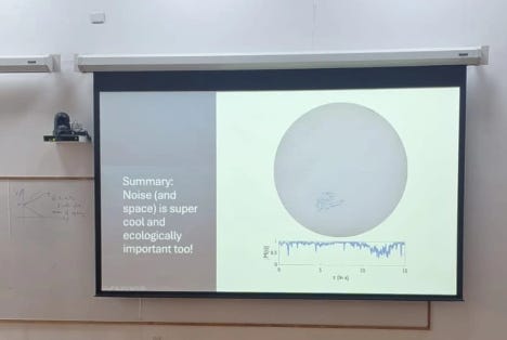
The talk was really insightful and message was; How cool is noise!
But isn’t noise suppose to be unpleasant? Well not really
As mentioned in the last blog, “Functions are deterministic. (By contrast, a relation in which you can get two different outputs from the same input is called stochastic)”
Deterministic models are approximations of real systems; a good model captures the signal (main deterministic trend) in the data. Never the less, the data likely will deviate somewhat from the model prediction. This deviation from the signal is called noise or stochasticity .The two main types of noise in biological data are process error and measurement error (observational error). The process error occurs because the real system is more complicated than the mathematical model. The measurement error occurs because the real system cannot be measured exactly (-Prof Ranjan Das).
There are two main types of process error in ecology: environmental stochasticity and demographic stochasticity. Stochastic events in a population can be likened to the toss of a fair coin. Imagine that a single coin is tossed for a population of animals. The outcome of the toss, although random, is the same for each individual member of the population. This is environmental stochasticity. Such extrinsic events as weather cause this type of noise. Now imagine that each animal in the population tosses its own coin. This time there is a random outcome for each individual. This is demographic stochasticity. Individual variability in intrinsic parameters such as birth and death rates cause this type of noise.
Systems in classical physics may have relatively little stochasticity, and their mathematical models can be so precise that some people call them “laws.” Some social science systems, on the other hand, may have a lot of stochasticity—so much so that the signal may be swamped out by noise and mathematical modeling may be impossible. In ecology, deterministic and stochastic forces are more or less equally important. Therefore, noise should ideally be incorporated explicitly into a deterministic model to produce a stochastic version of the model. The interaction of deterministic and stochastic forces can give rise to a rich class of emergent dynamic phenomena that cannot occur in purely deterministic or purely random systems.
Stochasticity is modeled mathematically through the notions of random variable and distribution. Suppose you count the number of seabirds on a beach (will look a paper, similar to this notion). If the number of birds is large, repeated counts of the exact same group of birds will probably yield different results due to observational error. We can use the notion of a random variable X to stand for the outcomes of trial observations (counts). Note that random variables are usually denoted with uppercase letters. A particular observation X = x, where x is an observed value, is called a realization of the random variable. You would want to know if some observations x are more likely than others, because you might want to know, for example, whether the count errors are biased. Mathematically, you would be asking, “what is the distribution of the random variable X?” The answer to this question is, of course, situation dependent. One has to make assumptions about how measurements, and hence errors, are distributed. Ideally, such assumptions can be tested experimentally.
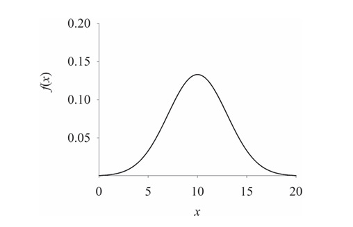
Different types of measurements have different limiting distributions. Nevertheless, a great many measurements are found to have a symmetrical bell-shaped curve for their limiting distribution.
The main distribution will be the normal distribution. Thanks to Prof Ranjan Das who taught us IDC202 ! We will continue our discussion by supposing the bird count random variable X is normally distributed about the true number of birds µ.
Here, f(x) is not the probability of observing x birds. Rather, the probability that the observational count X will fall between the values a and b is the area under the normal curve that lies between the vertical lines x = a and x = b; that is,
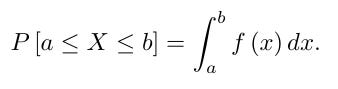
The total area under the normal curve gives the probability that the count lies between −∞ and +∞, which is, of course, equal to one. The expected value of the random variable X, often denoted E(X), is the sum of all possible outcomes of X weighted by the probability of obtaining that outcome. For the normal distribution, E[X] = µ The inflection points of the normal PDF f occur at x = µ±σ . The parameter σ is called the standard deviation. It measures the spread of the distribution about the mean µ. The square of the standard deviation, σ^2, is called the variance of the distribution.
I assume this much would be enough, we will see more while working with our hand-on experience of modelling.
With this post the series comes to an end, I am thinking to start a new series where we will start the actual modelling stuffs. Some of my friends have suggested to explore something apart from ecology like mathematical modelling at cellular level, so I am learning those for the moment. Meanwhile I would highly recommend to look after this blog, for mathematical oncology. It’s an evolving field and would love to learn together. See you all next time, till then.
Peace off !
Reference
Mathematical Modeling in Biology A Research Methods Approach Shandelle M. Henson and James L. Hayward
Lecture slides of IDC202
Insightful!
I missed to add that oncology blog! Here it is https://mathematical-oncology.org/blog/sysbio_video.html